hls4ml · measured

Benchmarks

Four benchmark models from the hls4ml literature mapped onto one XCK26 — what fits, what it costs, how far precision can drop, and how far the tool's estimates can be trusted.

Updated 2026-08-26

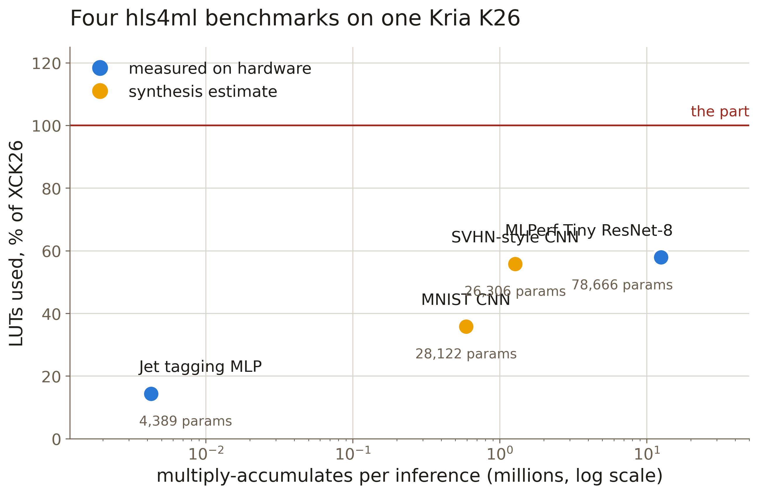
Four models from the hls4ml literature, on one part, so the numbers compare directly rather than across papers and devices. Two are deployed and measured on hardware; two are synthesized.

Model	Reference	Parameters	MMAC	Status
Jet tagging MLP	arXiv:1804.06913	4,389	0.004	on hardware
MNIST CNN	arXiv:2512.01463	28,122	0.59	synthesized
SVHN-style CNN	arXiv:2101.05108	26,306	1.27	synthesized
MLPerf Tiny ResNet-8	arXiv:2206.11791	78,666	12.50	on hardware

All at ap_fixed<16,6>, 100 MHz, xck26-sfvc784-2LV-c.

The SVHN model is trained on CIFAR-10. Same 32×32×3 input and ten classes, so its resource and latency figures are representative; its accuracy is not comparable to the published SVHN result and is not offered as such.

What fits

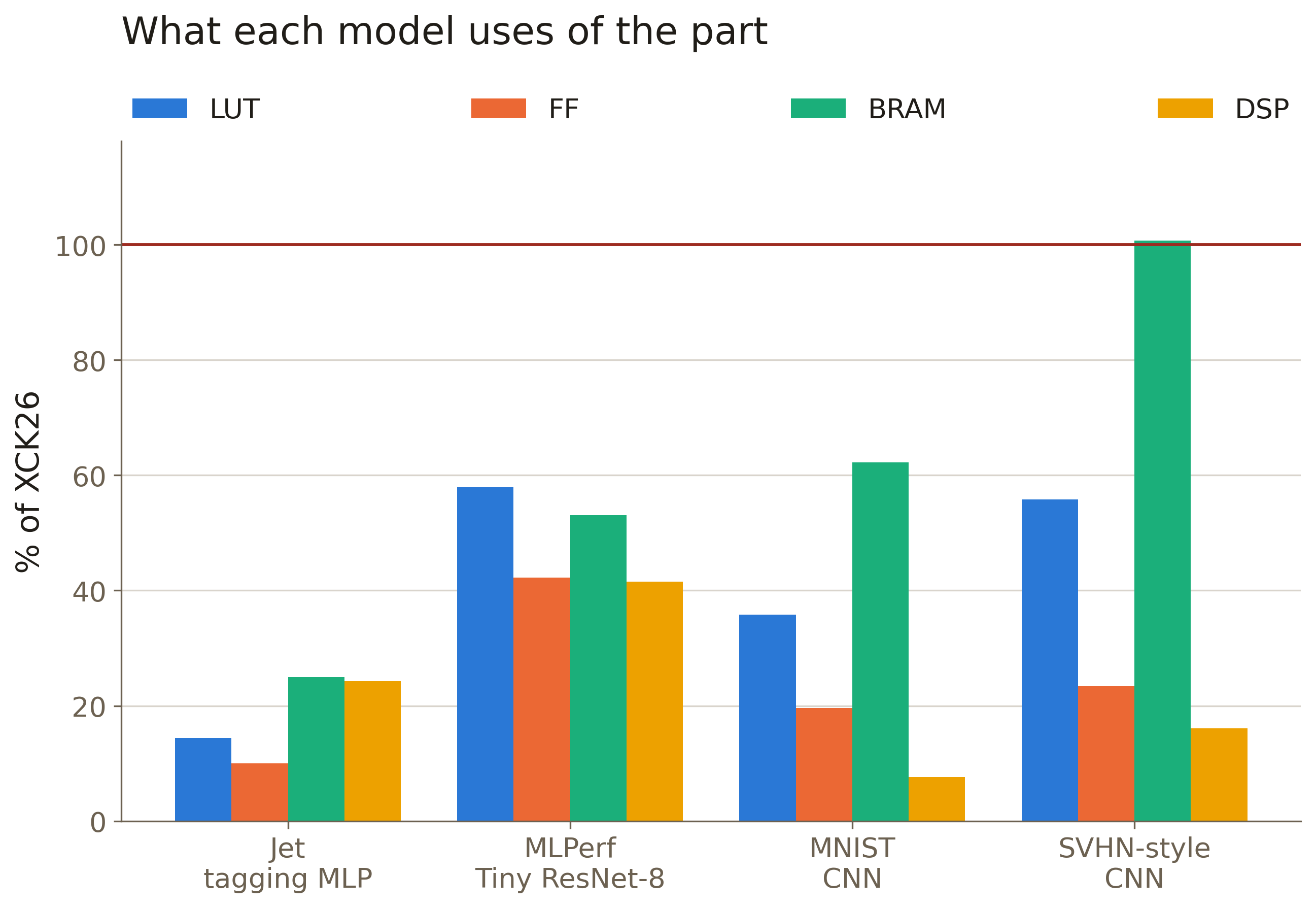
Four hls4ml benchmarks on one Kria K26 — LUT usage against arithmetic. Three orders of magnitude of model size, and the largest still uses under 60% of the part.

	LUT	FF	BRAM	DSP	Latency
Jet tagging MLP	14%	10%	25%	24%	3.2 µs
MNIST CNN	36%	20%	62%	8%	382 µs
SVHN-style CNN	56%	23%	101%	16%	694 µs
MLPerf Tiny ResNet-8	58%	42%	53%	42%	929 µs

Block RAM binds before DSPs do. The SVHN model wants 101% of block RAM while using 16% of the DSPs. Under io_stream, inter-layer FIFOs carry one channel vector per element, so their cost scales with width, not depth — a 64-channel stream is 1,024 bits wide and costs 29 BRAM18 even at depth 1. The K26’s 64 URAMs are the reserve for this case; binding the largest FIFOs to them moved one design from 173% block RAM to 93%.

What each model takes of the part. DSP usage stays low across the whole range; memory is the binding limit.

Latency

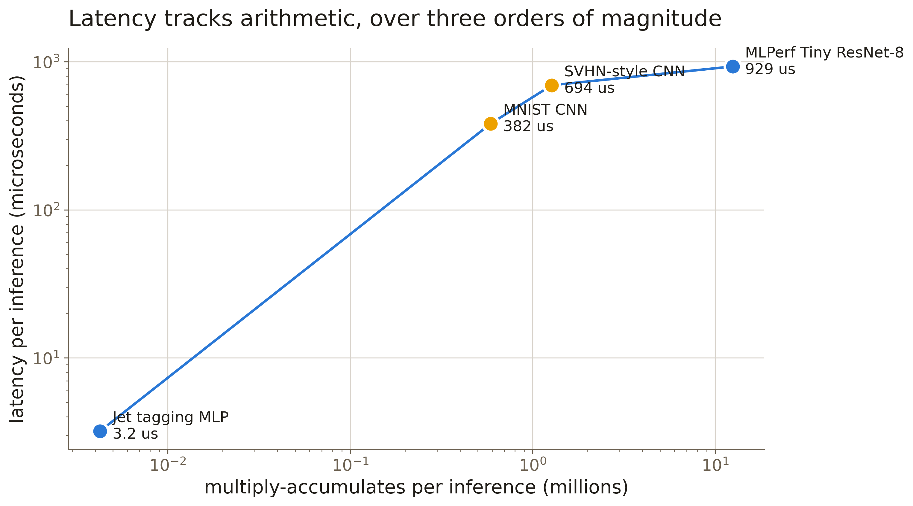
Latency follows arithmetic closely. The jet-tagging MLP at 3.2 µs is dominated by AXI register traffic rather than compute — its network finishes in 1.1 µs and the rest is bus. For everything larger, compute dominates and the interface disappears into the noise.

Precision

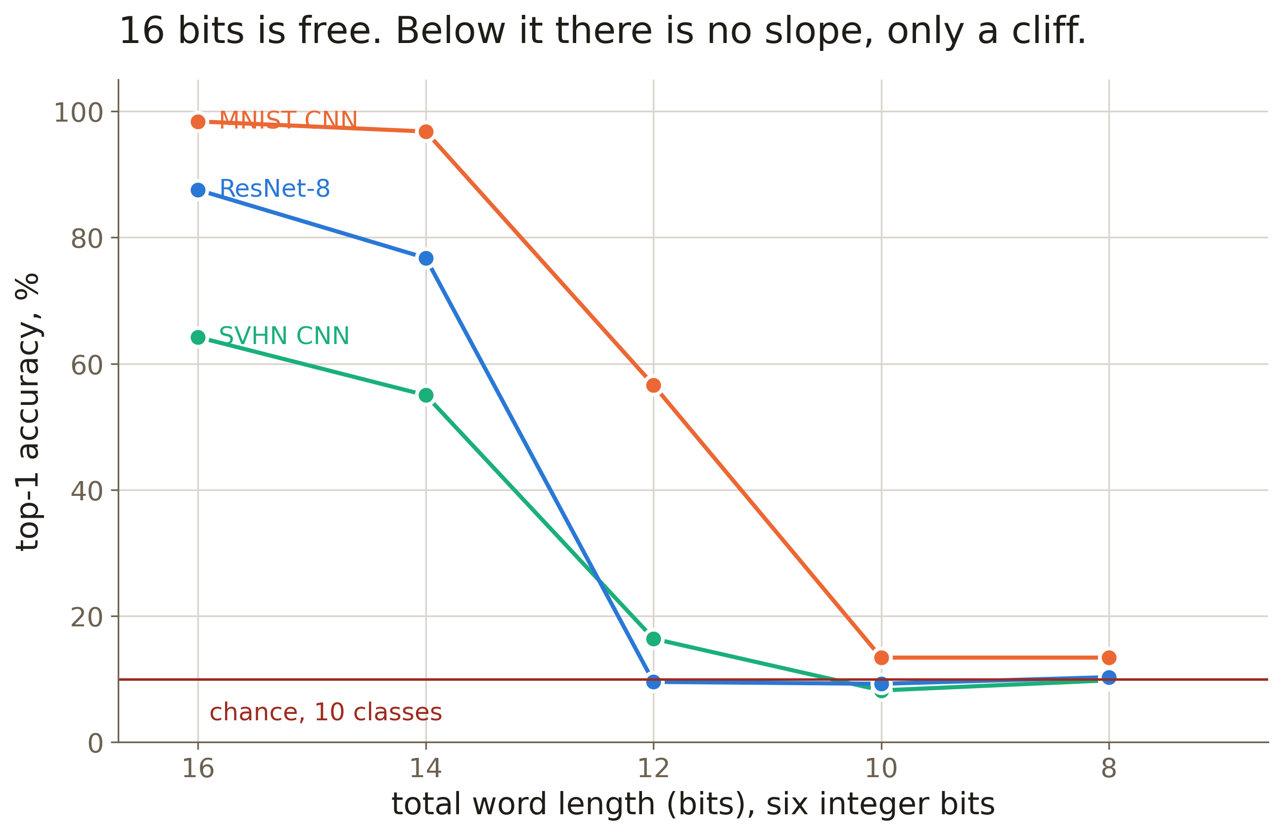
Bits	MNIST CNN	SVHN CNN	ResNet-8
float32	98.6%	65.2%	87.9%
16	98.4%	64.2%	87.6%
14	96.8%	55.0%	76.8%
12	56.6%	16.4%	9.6%
10	13.4%	8.2%	9.3%
8	13.4%	9.8%	10.3%

Sixteen bits is free and twelve is chance, with no useful ground in the middle. Every model in the suite behaves the same way, so this is a property of post-training quantization rather than of any one network. Budget resources at 16 bits, and if you need less, retrain for it — every published sub-16-bit hls4ml result uses quantization-aware training.

Accuracy end to end

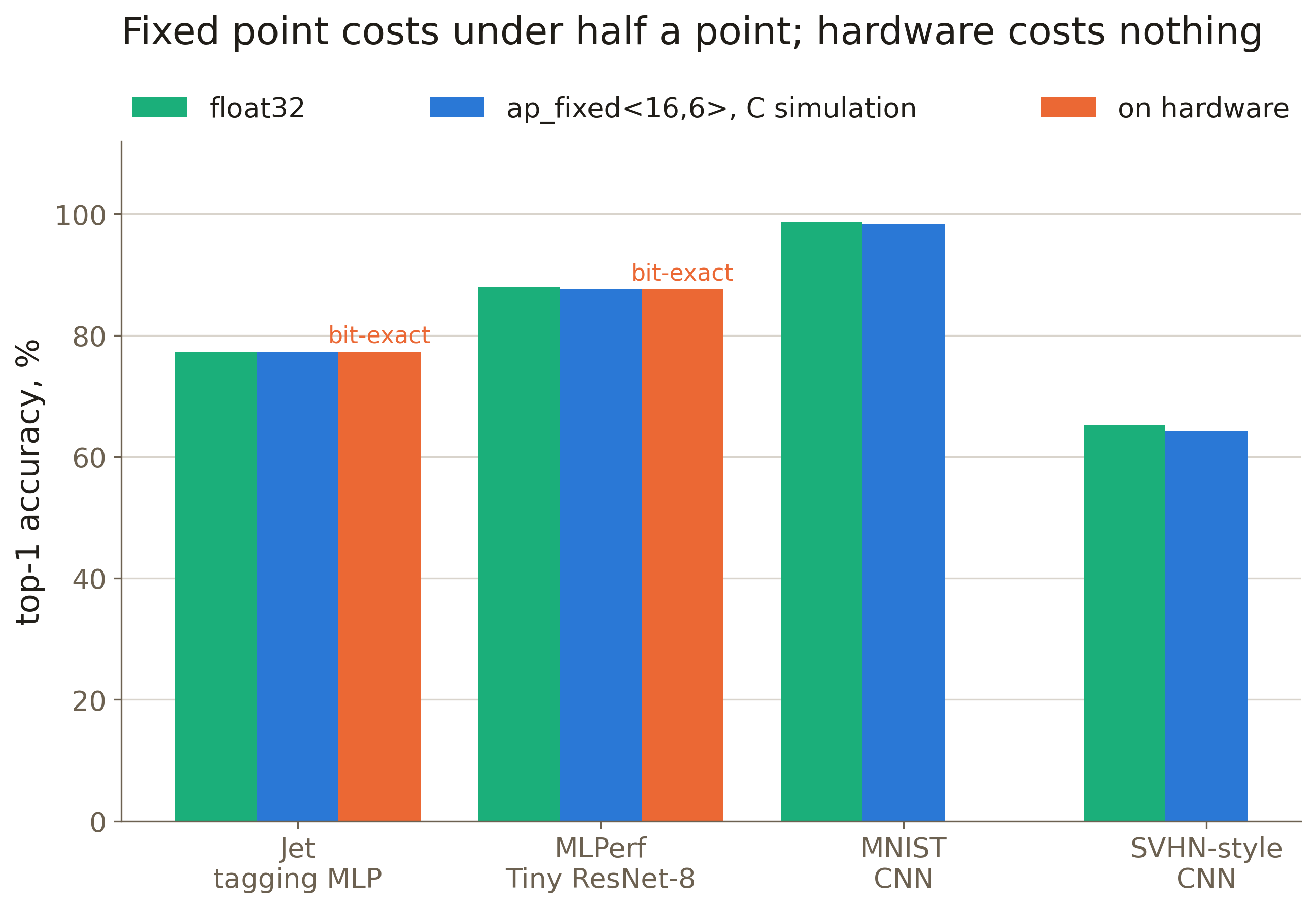
Accuracy through the flow — Float model, C simulation, and the fabric itself. Where a model is deployed, hardware reproduces the simulator exactly.

Fixed point costs under half a point. The fabric then costs nothing at all — both deployed models reproduce hls4ml’s C simulation bit for bit, 128 of 128 and 2,000 of 2,000 predictions identical with zero score difference.

That equality is the acceptance test worth running on a new model. Accuracy alone can match by coincidence; bit-exactness cannot, and it isolates a wrapper or driver fault from a network one.

How far to trust the estimates

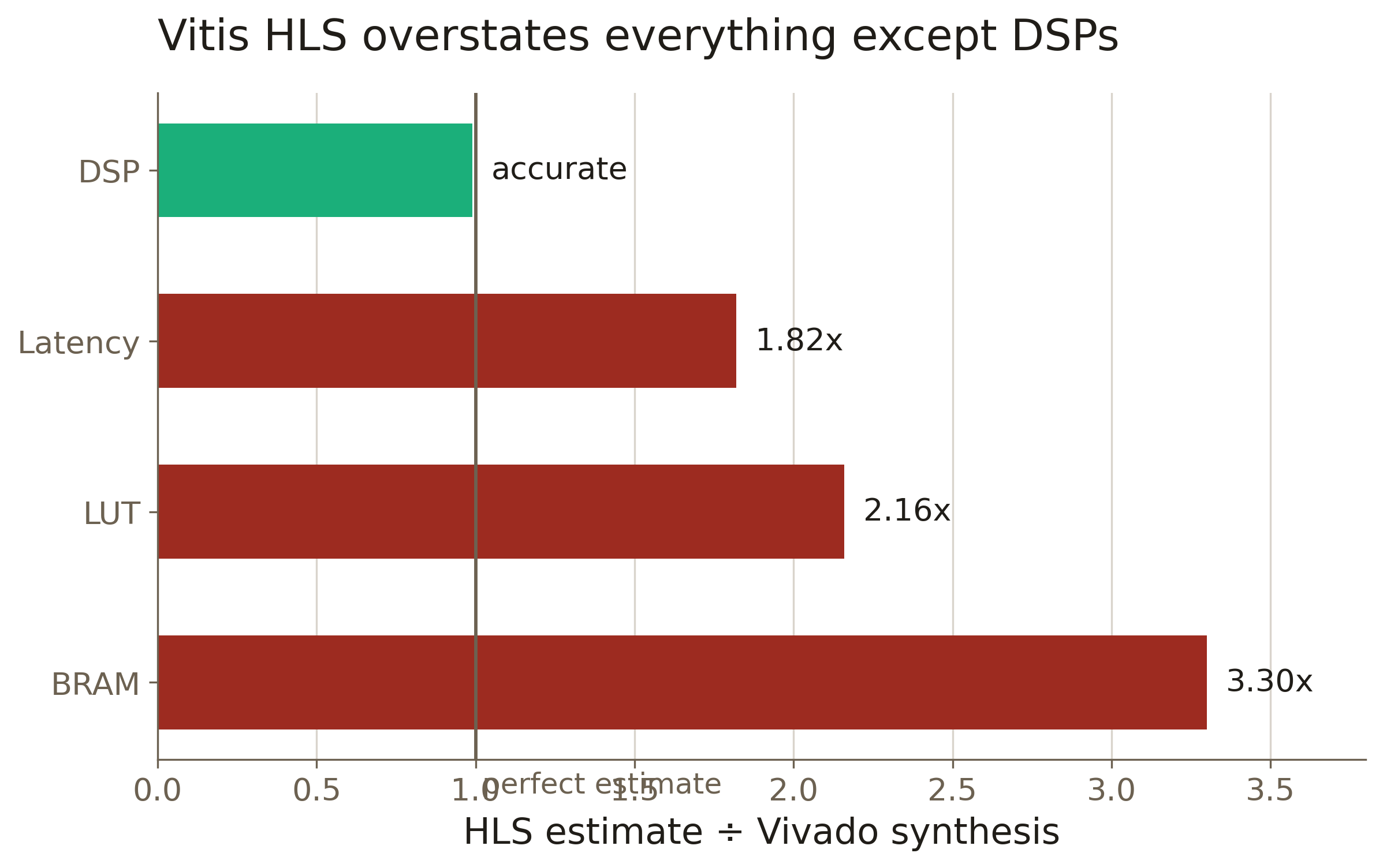
HLS estimate against Vivado synthesis — Measured on ResNet-8: the same design, high-level synthesis report against Vivado.

	HLS estimate ÷ Vivado
Block RAM	3.3×
LUT	2.2×
Latency	1.8×
DSP	accurate to 1%

This changes verdicts rather than decorating them. On the estimate, ResNet-8 misses the part; in reality it uses 58% of the LUTs and meets timing with 1.756 ns to spare. Always confirm with real synthesis before concluding a model does not fit — and note that published hls4ml resource figures are usually estimates of the same kind.

Where the logic goes

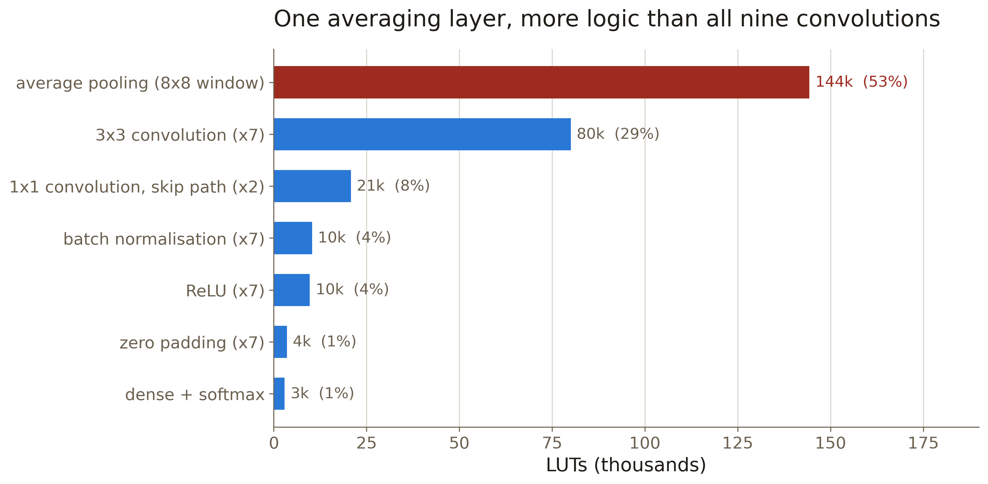
LUTs by layer kind — ResNet-8 as published. One 8×8 average-pooling layer costs more than all nine convolutions.

In the MLPerf reference model as published, a single 8×8 AveragePooling2D takes 52% of the LUTs and 61% of the flip-flops — 1.8× the cost of every convolution combined — because hls4ml’s streaming implementation buffers the whole window.

Where the pooling window covers the feature map, GlobalAveragePooling2D is the same arithmetic and accumulates as the stream goes past. Substituting it took the model from 237% of the part’s LUTs to 116%, with outputs matching to 1×10⁻⁶.

Reproducing this

cd sw/hls4ml/bench-suite
python models.py mnist svhn      # train the two that are not pretrained
./run_sweep.sh                   # precision sweep, then one synthesis per model
python collect.py                # merge into notebook/benchdata.json
jupyter nbconvert --to notebook --execute --inplace \
    notebook/krio_ml_benchmarks.ipynb

Figures land in notebook/figs/ as PNG at 300 dpi and PDF. Synthesis runs are serialized deliberately — two concurrent Vitis runs will exhaust a 30 GB machine.